arviz_plots.plot_energy#
- arviz_plots.plot_energy(dt, kind=None, threshold=0.3, sample_dims=None, plot_collection=None, backend=None, labeller=None, aes_by_visuals=None, visuals=None, stats=None, **pc_kwargs)[source]#
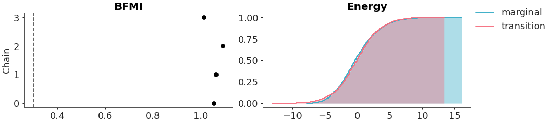
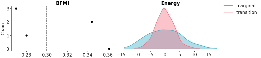
Plot energy distributions and bfmi from gradient-based algorithms.
Generate a figure with two plots: On the left the Bayesian Fraction of Missing Information (BFMI) per chain, values below the threshold indicate poor exploration of the energy distribution. On the right, the marginal energy distribution and the energy transition distribution. Ideally, these two distributions should overlap closely.
For details on BFMI and energy diagnostics see [1] for a more practical overview check the EABM chapter on MCMC diagnostic of gradient-based algorithms.
- Parameters:
- dt
xarray.DataTree sample_statsgroup with anenergyvariable is mandatory.- kind{“kde”, “hist”, “dot”, “ecdf”}, optional
How to represent the marginal density. Defaults to
rcParams["plot.density_kind"]- threshold
float, default 0.3 Reference threshold for BFMI values, values below this indicate poor exploration of the energy distribution.
- sample_dimssequence of
str, optional Dimensions to consider as sample dimensions when computing BFMI. Defaults to
rcParams["data.sample_dims"]- plot_collection
PlotCollection, optional - backend{“matplotlib”, “bokeh”, “plotly”}, optional
- labeller
labeller, optional - aes_by_visualsmapping of {
strsequence ofstr}, optional Mapping of visuals to aesthetics that should use their mapping in
plot_collectionwhen plotted. Valid keys are the same as forvisuals.- visualsmapping of {
strmapping or bool}, optional Valid keys are:
dist -> depending on the value of kind passed to:
“kde” -> passed to
line_xy“ecdf” -> passed to
ecdf_line“hist” -> passed to
step_hist“dot” -> passed to
scatter_xy
title -> passed to
labelled_titlelegend -> passed to
arviz_plots.PlotCollection.add_legendremove_axis -> not passed anywhere, can only be
Falseto skip calling this functiontitle -> passed to
labelled_titlebfmi_points -> passed to
scatter_xyfor BFMI scatter plotylabel -> passed to
labelled_yfor BFMI column y-axis labelface -> visual that fills the area under the energy distributions.
Defaults to True. Depending on the value of kind it is passed to:
“kde” or “ecdf” -> passed to
fill_between_y“hist” -> passed to
histdot -> ignored
- statsmapping, optional
Valid keys are:
dist -> passed to kde, ecdf, …
- **pc_kwargs
Passed to
arviz_plots.PlotCollection.wrap
- dt
- Returns:
References
[1]Betancourt. Diagnosing Suboptimal Cotangent Disintegrations in Hamiltonian Monte Carlo. (2016) https://arxiv.org/abs/1604.00695
Examples
Plot an energy plot using ecdf for the energy distributions.
>>> from arviz_plots import plot_energy, style
>>> style.use("arviz-variat")
>>> from arviz_base import load_arviz_data
>>> data = load_arviz_data('non_centered_eight')
>>> plot_energy(data, kind="ecdf")